TimescaleDB Tutorial: Real-Time Market Data to OHLC Candles Pipeline

Time-series data is the backbone of financial markets. Every tick, every price movement needs to be captured, stored, and aggregated efficiently. In this guide, we'll build a complete pipeline that ingests real-time market data and automatically aggregates it into OHLC (Open, High, Low, Close) candles at different timeframes using TimescaleDB.

Architecture Overview

Our pipeline consists of four layers:

Raw tick data ingestion - capturing every bid/ask update in a hypertable
One-minute continuous aggregate - pre-computed OHLC candles, auto-updated
Materialized one-minute table - separate persistent storage with custom job logic
Hourly continuous aggregate - higher timeframe built from 1-minute data

Tick to OHLC Map

Not interested in building infrastructure yourself, just try our subscription plan that does all the heavy lifting for you at no extra cost.

Why both a continuous aggregate AND a separate table? The continuous aggregate (tick_1m_view) handles most use cases efficiently. The separate ohlc_1m_table gives you flexibility for custom logic, external integrations, or specific business requirements.

Step 1: Create the Tick Data Hypertable

First, we'll create our raw tick data table and convert it to a TimescaleDB hypertable for optimized time-series storage.

-- Create the raw tick data table
CREATE TABLE tick_data (
    time TIMESTAMPTZ NOT NULL,
    symbol TEXT NOT NULL,
    bid NUMERIC(20, 8) NOT NULL,
    ask NUMERIC(20, 8) NOT NULL
);

-- Convert to hypertable (partitioned by time)
SELECT create_hypertable('tick_data', 'time');

-- Create index for symbol lookups
CREATE INDEX idx_tick_data_symbol_time ON tick_data (symbol, time DESC);

The hypertable automatically partitions data by time, making queries on recent data extremely fast while keeping historical data accessible.

Step 2: Insert Market Tick Data

Let's add some market data flowing in. We will show a small snippet to explain how to ingest data, for more info visit our docs page.

# Database connection
conn = psycopg2.connect(
    host="localhost",
    database="market_data",
    user="postgres",
    password="your_password"
)
conn.autocommit = True
cursor = conn.cursor()

def on_message(ws, message):
    """Handle incoming tick data"""
    try:
        data = json.loads(message)

        # TraderMade sends data in format: {"symbol":"EURUSD","ts":"1234567890123","bid":1.0512,"ask":1.0514}
        if 'symbol' in data and 'bid' in data and 'ask' in data:
            timestamp = datetime.fromtimestamp(int(data['ts']) / 1000)
            symbol = data['symbol']
            bid = float(data['bid'])
            ask = float(data['ask'])

            # Insert into tick_data table
            cursor.execute("""
                INSERT INTO tick_data (time, symbol, bid, ask)
                VALUES (%s, %s, %s, %s)
            """, (timestamp, symbol, bid, ask))

            print(f"{timestamp} | {symbol} | Bid: {bid} | Ask: {ask}")

Step 3: Create the One-Minute Continuous Aggregate

Here's where TimescaleDB really shines. Instead of a regular view that recomputes from raw ticks every time (inefficient!), we'll use a continuous aggregate. This materializes the aggregation results and automatically keeps them updated.

-- Create continuous aggregate for 1-minute OHLC with real-time aggregation
CREATE MATERIALIZED VIEW tick_1m_view
WITH (
    timescaledb.continuous,
    timescaledb.materialized_only = false  -- Enable real-time aggregation
) AS
SELECT
    time_bucket('1 minute', time) AS time,
    symbol,
    FIRST((bid + ask) / 2, time) AS open,
    MAX((bid + ask) / 2) AS high,
    MIN((bid + ask) / 2) AS low,
    LAST((bid + ask) / 2, time) AS close
FROM tick_data
GROUP BY time_bucket('1 minute', time), symbol;

Why continuous aggregates? - Pre-computed results stored on disk (not recalculated each query) - Automatically updated as new data arrives - Orders of magnitude faster than regular views on large datasets - Can serve millions of queries without touching raw tick data

Add a refresh policy to keep it updated:

-- Refresh the last 2 hours of data every minute
SELECT add_continuous_aggregate_policy('tick_1m_view',
    start_offset => INTERVAL '1 hour',
    end_offset => INTERVAL '1 minute',
    schedule_interval => INTERVAL '1 minute');

Query it just like a regular table:

SELECT * FROM tick_1m_view 
WHERE symbol = 'EURUSD' 
ORDER BY time DESC 
LIMIT 10;

Step 4: Create the Materialized One-Minute Table

Views are computed on-the-fly, which can be slow for large datasets. We'll create a materialized table that stores pre-computed one-minute candles.

-- Create the materialized OHLC table
CREATE TABLE ohlc_1m_table (
    time TIMESTAMPTZ NOT NULL,
    symbol TEXT NOT NULL,
    open NUMERIC(20, 8) NOT NULL,
    high NUMERIC(20, 8) NOT NULL,
    low NUMERIC(20, 8) NOT NULL,
    close NUMERIC(20, 8) NOT NULL,
    PRIMARY KEY (time, symbol)
);

-- Convert to hypertable
SELECT create_hypertable('ohlc_1m_table', 'time');

-- Create index for efficient symbol queries
CREATE INDEX idx_ohlc_1m_symbol_time ON ohlc_1m_table (symbol, time DESC);

Step 5: Create the Automated Refresh Job

This is where the magic happens. We'll create a TimescaleDB job that runs every minute, aggregating the last 2 minutes of data from our view into the materialized table. The ON CONFLICT clause ensures we update existing records if they already exist.

-- Create the procedure that will be run by the job
CREATE OR REPLACE PROCEDURE refresh_ohlc_1m()
LANGUAGE SQL
AS $$
    INSERT INTO ohlc_1m_table (time, symbol, open, high, low, close)
    SELECT time, symbol, open, high, low, close
    FROM tick_1m_view
    WHERE time >= DATE_TRUNC('minute', NOW()) - INTERVAL '2 minutes'
    ON CONFLICT (time, symbol)
    DO UPDATE SET
        open = EXCLUDED.open,
        high = EXCLUDED.high,
        low = EXCLUDED.low,
        close = EXCLUDED.close;
$$;

-- Schedule the job to run every minute
SELECT add_job('refresh_ohlc_1m', '1 minute');

Why 2 minutes? This provides a buffer to capture late-arriving ticks and ensures the previous minute's candle is finalized while starting to build the current one.

You can manually test the procedure:

CALL refresh_ohlc_1m();
SELECT * FROM ohlc_1m_table ORDER BY time DESC LIMIT 5;

Step 6: Create the One-Hour Continuous Aggregate (this procedeure can be followed for any timeframe)

Similarly, create an hourly continuous aggregate from the one-minute data. Notice we're building on top of the continuous aggregate, not the raw tick data - this is the efficient hierarchical approach.

-- Create continuous aggregate for 1-hour OHLC
CREATE MATERIALIZED VIEW ohlc_1h_view
WITH (
    timescaledb.continuous,
    timescaledb.materialized_only = false  -- Enable real-time aggregation
) AS
SELECT
    time_bucket('1 hour', time) AS time,
    symbol,
    FIRST(open, time) AS open,
    MAX(high) AS high,
    MIN(low) AS low,
    LAST(close, time) AS close
FROM ohlc_1m_table  -- Building from the materialized 1-minute table
GROUP BY time_bucket('1 hour', time), symbol;

-- Add refresh policy for hourly data
SELECT add_continuous_aggregate_policy('ohlc_1h_view',
    start_offset => INTERVAL '24 hours',
    end_offset => INTERVAL '1 hour',
    schedule_interval => INTERVAL '30 minutes');

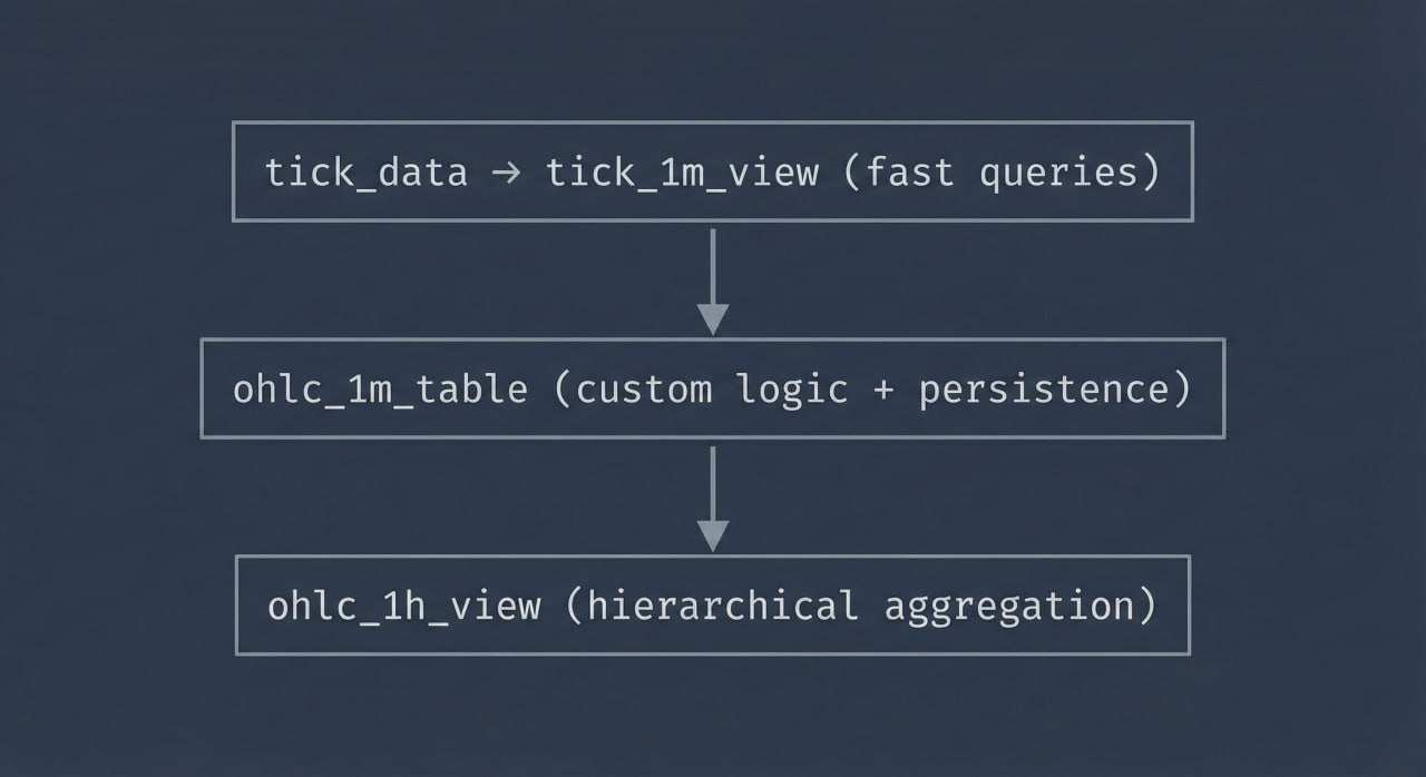
Performance benefit: The hourly aggregate reads from the pre-computed 1-minute data (60 rows) instead of potentially thousands of raw ticks. This creates a fast, scalable hierarchy:

tick_data → tick_1m_view (fast queries)
              ↓
         ohlc_1m_table (custom logic + persistence)
              ↓
         ohlc_1h_view (hierarchical aggregation)

Query the hourly data:

SELECT * FROM ohlc_1h_view 
WHERE symbol = 'EURUSD' 
ORDER BY time DESC 
LIMIT 24;

Monitoring and Management

Check your continuous aggregates and jobs:

-- View all continuous aggregates
SELECT * FROM timescaledb_information.continuous_aggregates;

-- View all jobs (including continuous aggregate refresh policies)
SELECT * FROM timescaledb_information.jobs;

-- View job statistics
SELECT * FROM timescaledb_information.job_stats;

Data Retention Policies

Automatically drop old data to manage storage:

-- Drop tick data older than 30 days
SELECT add_retention_policy('tick_data', INTERVAL '30 days');

-- Keep OHLC data for 2 years
SELECT add_retention_policy('ohlc_1m_table', INTERVAL '2 years');

Conclusion

You now have a production-ready pipeline that:

Ingests real-time tick data efficiently into a hypertable
Uses continuous aggregates for fast, pre-computed OHLC candles (not slow views!)
Maintains a separate materialized table for custom business logic
Provides hierarchical aggregation (minute → hour) for scalability
Includes retention policies for long-term storage
Automatically refreshes aggregations as new data arrives

Key takeaway: Continuous aggregates are the secret sauce. They give you the convenience of views with the performance of materialized tables, automatically maintained by TimescaleDB.

This architecture scales to millions of ticks per day. The query performance difference is dramatic:

Regular view on 1M ticks: ~2-5 seconds
Continuous aggregate: ~10-50ms (100x+ faster!)

You can easily expand this architecture with additional timeframes—such as 5m, 15m, 4h, or 1d—by creating more continuous aggregates. You can also apply compression and leverage other Timescale features for even greater efficiency. Altogether, this setup transforms raw tick data into a scalable, high-performance analytics and data delivery engine.

The 6-Step Blueprint: Real-time Market Data Pipeline with TimescaleDB