Real-Time Market Data Monitoring with Grafana, PostgreSQL, TimescaleDB, and Docker

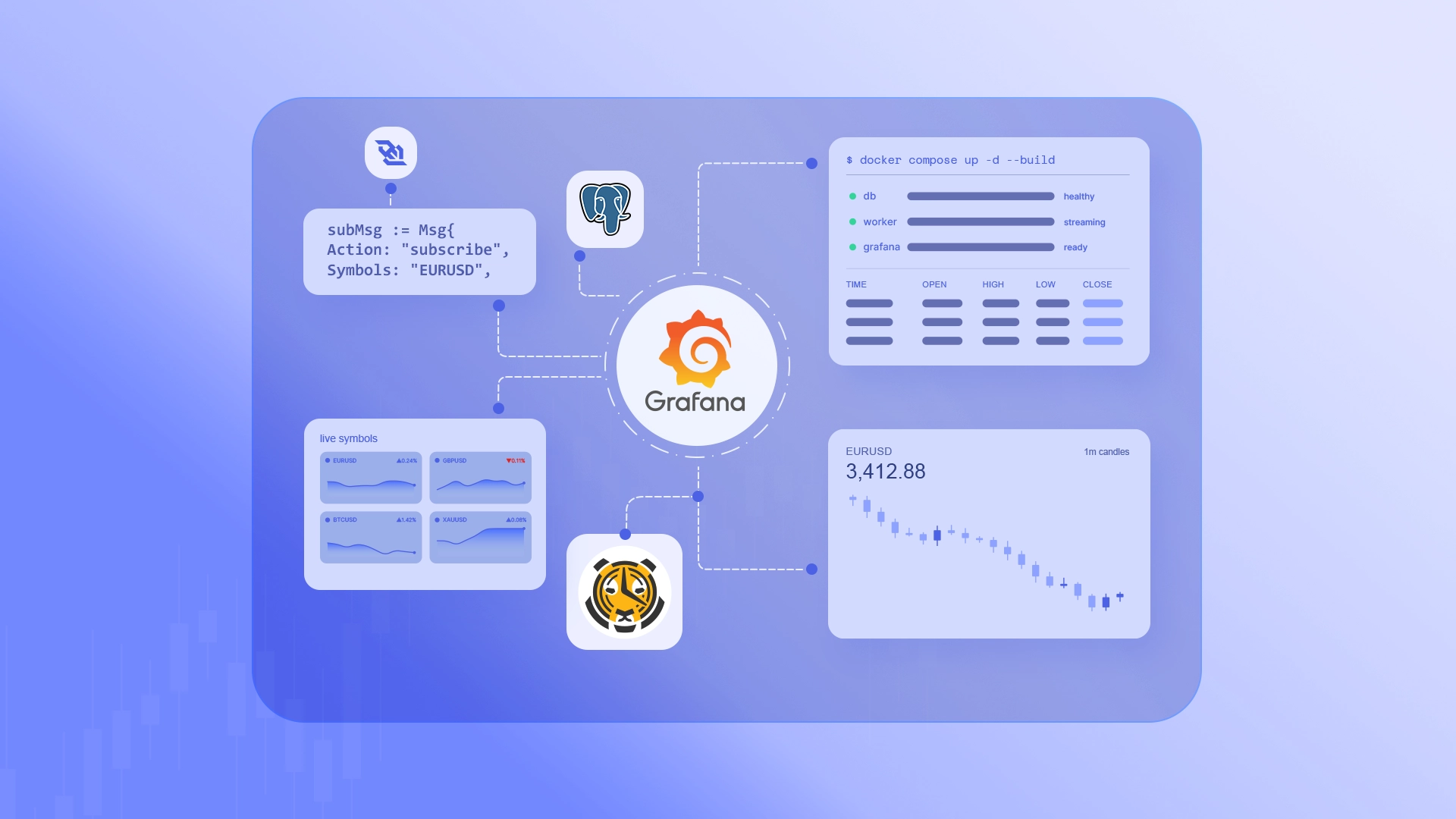
This tutorial builds a reproducible local monitoring stack for real-time market data. TraderMade prices — FX and US stocks — arrive over a WebSocket connection, an ingestion worker persists each tick to PostgreSQL, TimescaleDB maintains one-minute OHLC aggregates, and Grafana renders the result as an automatically refreshing candlestick chart.

The worker is shown in Python here, but the ingestion engine can be written in any language: its only contract is to authenticate, subscribe, and insert each quote into the raw tick table. Any language with a WebSocket client and a PostgreSQL driver — Go, Node.js, Rust, Java, C#, or others — works equally well.

The complete stack runs under Docker Compose and starts with a single command.

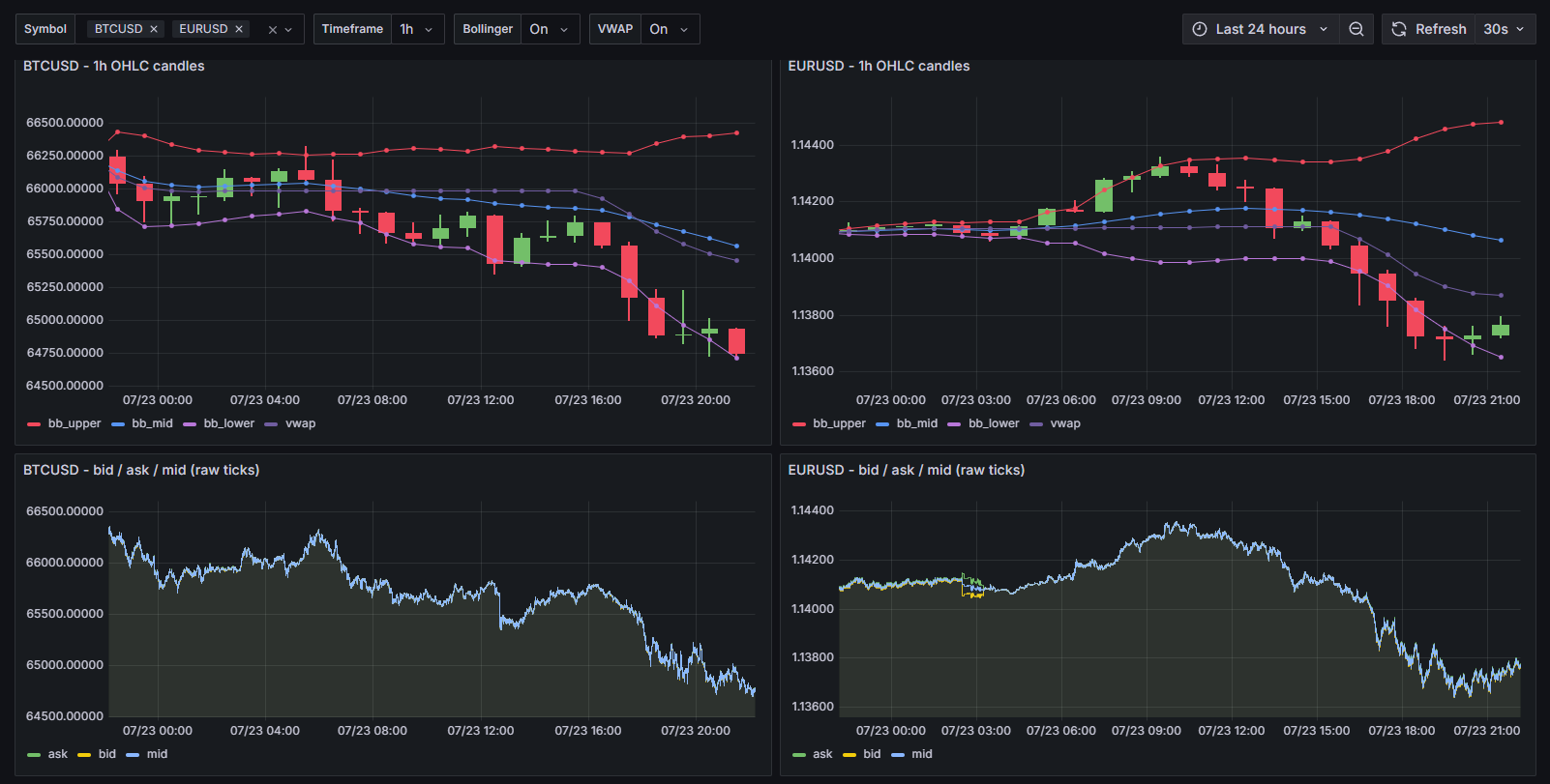
Live candlestick dashboard in Grafana

Persisting the stream changes it from an ephemeral terminal feed into an operational dataset that can be queried, aggregated, visualised, and retained independently of the client process — the foundation of any algorithmic trading, backtesting, or market-analytics infrastructure.

This guide complements the 6-step TimescaleDB pipeline tutorial, which defines the raw tick hypertable and the continuous aggregate used to produce OHLC candles. Here, you will package that data pipeline with a live ingestion worker and a provisioned Grafana dashboard.

The complete project is available in the companion repository; you can clone it to run the full stack directly, or follow the steps below to build it yourself.

Architecture

The stack contains three services:

TimescaleDB stores raw ticks and maintains the prices_1m continuous aggregate.
Ingestion worker subscribes to the TraderMade WebSocket API and inserts each quote into PostgreSQL (Python here, any language in practice).
Grafana queries the aggregate and renders a live candlestick panel.

Docker Compose provides service discovery, startup ordering, persistent volumes, and a repeatable local runtime.

What you will build

By the end of the tutorial, you will have:

A PostgreSQL 16 database with the TimescaleDB extension
A WebSocket ingestion service (implemented here in Python, portable to any language)
A Docker Compose definition for the complete stack
A Grafana data source and dashboard managed as code
A symbol-selectable, auto-refreshing one-minute candlestick chart

Prerequisites

You should be comfortable reading Python, SQL, YAML, and Dockerfiles. Prior experience with Grafana or TimescaleDB is useful but not required.

You will also need:

Docker Desktop 4.x, or Docker Engine 24+ with Compose v2
A TraderMade API key with streaming enabled from your dashboard
A shell with docker and docker compose available

Verify the Docker installation before continuing:

docker --version
docker compose version

Your streaming WebSocket key may differ from your REST API key.

Step 1: Create the project structure

Create the project directory and the folders required by the three services:

mkdir market-monitor && cd market-monitor
mkdir -p db worker backfill grafana/provisioning/datasources grafana/provisioning/dashboards grafana/dashboards

The completed project will use the following structure:

market-monitor/
├── docker-compose.yml       # service definitions and shared runtime configuration
├── .env                     # API key and database configuration
├── db/
│   └── init.sql             # TimescaleDB schema and continuous aggregate
├── worker/
│   ├── Dockerfile
│   ├── requirements.txt
│   └── stream_to_db.py      # WebSocket ingestion worker
├── backfill/                # optional REST gap-backfill service (see repository)
└── grafana/
    ├── provisioning/        # provisioned data source and dashboard provider
    └── dashboards/          # version-controlled Grafana dashboards

Step 2: Add the TimescaleDB schema

The database requires two objects:

A raw-tick hypertable for incoming quotes
A one-minute OHLC continuous aggregate named prices_1m

Both are defined in the 6-step TimescaleDB pipeline tutorial, and the ready-to-use script is in the companion repository. Copy it from the repository or build it from the tutorial, and save it as:

db/init.sql

The TimescaleDB container executes files in /docker-entrypoint-initdb.d/ when it initialises a new data directory. Confirm that db/init.sql creates both the prices hypertable and the prices_1m continuous aggregate, because Grafana will query those objects directly.

Step 3: Implement the streaming worker

Start with the client from the Python WebSocket tutorial, which covers authentication, subscription, and message handling. Extend it with a PostgreSQL connection and an insert for each quote frame.

The complete, self-contained worker is shown below. It opens the WebSocket, logs in, subscribes to each symbol's QUOTE channel, and writes every quote frame to the prices table. Database configuration comes from the same environment variables as Docker Compose. Save it as worker/stream_to_db.py:

import json
import os
from datetime import datetime, timezone

import psycopg2
import websocket

API_KEY = os.environ["TM_API_KEY"]
SYMBOLS = [s.strip() for s in os.getenv("TM_SYMBOLS", "EURUSD,GBPUSD,BTCUSD,XAUUSD").split(",") if s.strip()]

WS_URL = "wss://stream.tradermade.com/feedAdv"

db = psycopg2.connect(
    host=os.getenv("POSTGRES_HOST", "db"),
    dbname=os.getenv("POSTGRES_DB", "marketdata"),
    user=os.getenv("POSTGRES_USER", "tm"),
    password=os.getenv("POSTGRES_PASSWORD", "tm"),
)
db.autocommit = True
cur = db.cursor()


def parse_ts(ts):
    # TraderMade timestamps are UTC in the form YYYYMMDD-HH:MM:SS.mmm
    return datetime.strptime(ts, "%Y%m%d-%H:%M:%S.%f").replace(tzinfo=timezone.utc)


def on_open(ws):
    # Authenticate as soon as the socket opens.
    ws.send(json.dumps({"action": "login", "key": API_KEY, "fmt": "JSON"}))


def on_message(ws, raw):
    try:
        msg = json.loads(raw)
    except ValueError:
        return  # non-JSON control text such as "Connected"

    # Once login is accepted, subscribe to each symbol's QUOTE channel.
    if msg.get("message") == "login_ok":
        channels = [f"{s}:QUOTE" for s in SYMBOLS]
        ws.send(json.dumps({"action": "subscribe", "symbols": channels, "send_last": True}))
        print(f"login ok — subscribing to {channels}", flush=True)
        return

    # Persist each QUOTE frame. The feed also carries bid/ask volume (bv, av)
    # if you later want a volume-weighted VWAP; this schema stores prices only.
    if msg.get("t") == "QUOTE" and "b" in msg and "a" in msg:
        bid = float(msg["b"])
        ask = float(msg["a"])
        mid = (bid + ask) / 2
        cur.execute(
            """
            INSERT INTO prices (symbol, bid, ask, mid, ts)
            VALUES (%s, %s, %s, %s, %s)
            """,
            (msg["s"], bid, ask, mid, parse_ts(msg["ts"])),
        )


def on_error(ws, error):
    print(f"[ws] error: {error}", flush=True)


def on_close(ws, status_code, reason):
    print(f"[ws] closed: {status_code} {reason}", flush=True)


if __name__ == "__main__":
    ws = websocket.WebSocketApp(
        WS_URL,
        on_open=on_open,
        on_message=on_message,
        on_error=on_error,
        on_close=on_close,
    )
    # run_forever auto-reconnects if the connection drops; ping keeps it alive.
    ws.run_forever(ping_interval=20, ping_timeout=10, reconnect=5)

The ingestion boundary is intentionally narrow: the worker authenticates, subscribes, normalises each quote, and writes it to the raw tick table. Aggregation remains a database concern, and visualisation a Grafana concern. Because that boundary is so small, you can swap Python for any language with a WebSocket client and a PostgreSQL driver — adjust worker/Dockerfile accordingly, and the rest of the stack is unchanged.

Create worker/requirements.txt:

websocket-client==1.8.0
psycopg2-binary==2.9.10

Create worker/Dockerfile:

FROM python:3.12-slim

WORKDIR /app

COPY requirements.txt .
RUN pip install --no-cache-dir -r requirements.txt

COPY stream_to_db.py .

ENV PYTHONUNBUFFERED=1

CMD ["python", "stream_to_db.py"]

The pinned dependencies make local builds repeatable. For a production deployment, add connection retry logic, WebSocket reconnection with backoff, structured logging, and graceful shutdown handling to the worker.

Step 4: Define the stack with Docker Compose

Create docker-compose.yml in the project root:

services:
  db:
    image: timescale/timescaledb:2.17.2-pg16
    environment:
      POSTGRES_USER: ${POSTGRES_USER:-tm}
      POSTGRES_PASSWORD: ${POSTGRES_PASSWORD:-tm}
      POSTGRES_DB: ${POSTGRES_DB:-marketdata}
    ports:
      - "5432:5432"
    volumes:
      - pgdata:/var/lib/postgresql/data
      - ./db/init.sql:/docker-entrypoint-initdb.d/init.sql:ro
    healthcheck:
      test: ["CMD-SHELL", "pg_isready -U ${POSTGRES_USER:-tm} -d ${POSTGRES_DB:-marketdata}"]
      interval: 3s
      timeout: 3s
      retries: 10

  worker:
    build: ./worker
    depends_on:
      db:
        condition: service_healthy
    environment:
      TM_API_KEY: ${TM_API_KEY:?set TM_API_KEY in your .env file}
      TM_SYMBOLS: ${TM_SYMBOLS:-EURUSD,GBPUSD,BTCUSD,XAUUSD}
      POSTGRES_HOST: db
      POSTGRES_USER: ${POSTGRES_USER:-tm}
      POSTGRES_PASSWORD: ${POSTGRES_PASSWORD:-tm}
      POSTGRES_DB: ${POSTGRES_DB:-marketdata}
    restart: unless-stopped

  grafana:
    image: grafana/grafana:11.3.0
    depends_on:
      db:
        condition: service_healthy
    ports:
      - "3001:3000"
    environment:
      POSTGRES_USER: ${POSTGRES_USER:-tm}
      POSTGRES_PASSWORD: ${POSTGRES_PASSWORD:-tm}
      POSTGRES_DB: ${POSTGRES_DB:-marketdata}
      GF_AUTH_ANONYMOUS_ENABLED: "true"
      GF_AUTH_ANONYMOUS_ORG_ROLE: "Admin"
      GF_AUTH_DISABLE_LOGIN_FORM: "true"
    volumes:
      - ./grafana/provisioning:/etc/grafana/provisioning:ro
      - ./grafana/dashboards:/var/lib/grafana/dashboards:ro
      - grafana-data:/var/lib/grafana
    restart: unless-stopped

volumes:
  pgdata:
  grafana-data:

The configuration establishes several important runtime behaviours:

Pinned images: TimescaleDB and Grafana use explicit image tags rather than floating versions.
Build isolation: The worker is built from worker/Dockerfile; the database and dashboard use published images.
Fail-fast configuration: ${TM_API_KEY:?...} prevents the stack from starting without a streaming API key.
Readiness gating: The worker and Grafana start only after pg_isready reports that PostgreSQL is accepting connections.
Service discovery: Compose provides an internal DNS entry for each service, so both clients connect to the database at db:5432.
Persistent state: The pgdata and grafana-data volumes survive container replacement and restarts.
Host access: PostgreSQL is exposed on localhost:5432. If a local PostgreSQL already uses that port, remap the host side (see Troubleshooting).

depends_on controls startup ordering; it does not provide runtime recovery if PostgreSQL later becomes unavailable. The worker should still implement retry and reconnect behaviour before this pattern is used outside local development.

Create .env in the project root:

TM_API_KEY=your_streaming_api_key_here
TM_SYMBOLS=EURUSD,GBPUSD,BTCUSD,XAUUSD
POSTGRES_USER=tm
POSTGRES_PASSWORD=tm
POSTGRES_DB=marketdata

Replace your_streaming_api_key_here with the streaming key from your TraderMade dashboard.

Add .env to .gitignore and do not commit credentials to source control.

Local development only: The Grafana configuration enables anonymous access with the Admin role and disables the login form. Do not expose this configuration on a shared network or use it in production.

Step 5: Provision the Grafana data source

Provisioning the data source in code avoids manual configuration and ensures every environment starts with the same connection definition.

Create the file below:

grafana/provisioning/datasources/datasource.yml

apiVersion: 1

datasources:
  - name: MarketData
    uid: marketdata
    type: postgres
    access: proxy
    url: db:5432
    user: ${POSTGRES_USER}
    isDefault: true
    jsonData:
      database: ${POSTGRES_DB}
      sslmode: disable
      postgresVersion: 1600
    secureJsonData:
      password: ${POSTGRES_PASSWORD}

Grafana resolves db through the Compose network and connects to PostgreSQL on its internal port. SSL is disabled because traffic remains inside the local Docker network.

Next, create the file below:

grafana/provisioning/dashboards/dashboards.yml

apiVersion: 1

providers:
  - name: TraderMade
    type: file
    options:
      path: /var/lib/grafana/dashboards

This provider instructs Grafana to load dashboard definitions from the mounted grafana/dashboards directory. The data source and dashboards can now be reviewed, versioned, and deployed with the rest of the project.

Step 6: Define the candlestick dashboard

Grafana's built-in Candlestick panel expects time-series rows containing time, open, high, low, and close. The prices_1m continuous aggregate already exposes those fields.

Create grafana/dashboards/marketdata.json:

{
  "title": "Market Monitor",
  "uid": "market-monitor",
  "schemaVersion": 39,
  "refresh": "5s",
  "time": { "from": "now-30m", "to": "now" },
  "templating": {
    "list": [
      {
        "name": "symbol",
        "type": "query",
        "label": "Symbol",
        "datasource": { "type": "postgres", "uid": "marketdata" },
        "query": "SELECT DISTINCT symbol FROM prices ORDER BY 1",
        "refresh": 2
      }
    ]
  },
  "panels": [
    {
      "id": 1,
      "title": "$symbol — 1-minute candles",
      "type": "candlestick",
      "datasource": { "type": "postgres", "uid": "marketdata" },
      "gridPos": { "h": 14, "w": 24, "x": 0, "y": 0 },
      "targets": [
        {
          "refId": "A",
          "format": "table",
          "rawQuery": true,
          "rawSql": "SELECT bucket AS \"time\", open, high, low, close FROM prices_1m WHERE symbol = ${symbol:sqlstring} AND $__timeFilter(bucket) ORDER BY bucket"
        }
      ]
    }
  ]
}

Two Grafana features drive the dashboard interaction:

${symbol:sqlstring} substitutes the selected symbol using Grafana's SQL string formatting.
$__timeFilter(bucket) constrains the query to the dashboard's active time range.

The dashboard refreshes every five seconds, while the underlying aggregate produces one-minute candles.

Step 7: Start and validate the stack

Build and start all services from the project root:

docker compose up -d --build

Inspect the worker logs:

docker compose logs -f worker

After authentication and subscription, the worker should begin persisting quote frames:

worker-1  | login ok — subscribing to ['EURUSD:QUOTE', 'GBPUSD:QUOTE', 'BTCUSD:QUOTE', 'XAUUSD:QUOTE']
worker-1  | [db] storing ticks...

Press Ctrl+C to stop following the logs; the container continues running in the background.

Open http://localhost:3001, select a symbol, and allow enough time for the first complete one-minute candle to be materialised.

You can validate the aggregate independently of Grafana by querying PostgreSQL directly:

docker compose exec db psql -U tm -d marketdata -c \
  "SELECT bucket, symbol, open, high, low, close, ticks FROM prices_1m WHERE symbol='BTCUSD' ORDER BY bucket DESC LIMIT 5;"

Example output:

        bucket         | symbol |   open   |   high   |   low    |  close   | ticks
-----------------------+--------+----------+----------+----------+----------+-------
 2026-07-22 12:37:00+00| BTCUSD | 65818.93 | 65823.28 | 65805.09 | 65819.96 |   200
 2026-07-22 12:36:00+00| BTCUSD | 65798.31 | 65824.91 | 65795.83 | 65819.09 |   453

This query confirms the complete path independently: ticks are being ingested, the continuous aggregate is producing OHLC rows, and the data required by Grafana is available.

Additional features

The following features are optional and independent. Each is a small addition to the provisioned dashboard or a companion service. The configuration and code are in the companion repository.

Select the candlestick timeframe

A Timeframe selector switches the candles between 1m, 5m, 15m, 30m, 1h, 2h, and 1d. Higher timeframes are re-bucketed from prices_1m on demand, so no extra tables or aggregates are required. Widen the dashboard time range to suit the timeframe, for example Last 24 hours for 1h.

The 5s-style control at the top right is Grafana's refresh rate, not the candle timeframe.

Overlay Bollinger Bands and a VWAP line

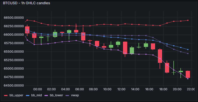
Two On/Off toggles draw indicators over the candles:

Bollinger Bands — a 20-period moving average with bands at plus and minus two standard deviations.
VWAP — a tick-weighted average price. This tutorial does not use traded volume: the WebSocket feed can carry volume, which the worker could capture into the database and feed into a true volume-weighted VWAP, but we have left that out to keep the stack simple. The result is therefore an activity-weighted approximation rather than a volume-weighted VWAP.

Bollinger Bands and a VWAP

Compare every symbol at once

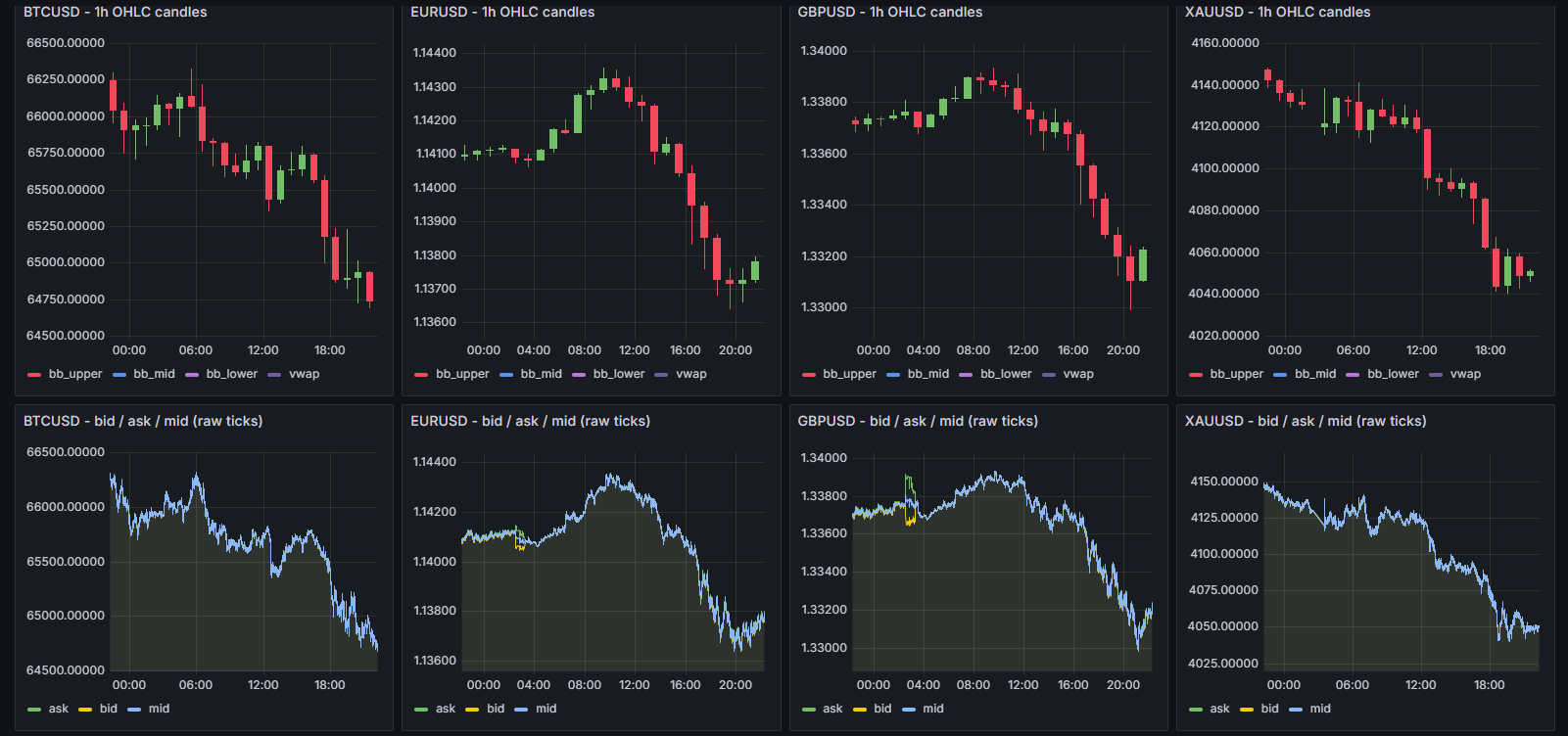
An All option on the symbol selector shows every instrument together, one candlestick panel per symbol, each with its own price axis. Separate axes are necessary because instruments trade at very different levels, such as BTCUSD near 65,000 and EURUSD near 1.14.

Multiple Symbol

Backfill missing history from the REST API

If the worker stops, no ticks are stored for that period and the candles show a gap. A small backfill service reconciles this from the TraderMade REST timeseries endpoint: it detects the gaps, fetches the missing one-minute history, and writes it back so the candles rebuild. Minutes that genuinely have no data, such as weekends and the daily metals break, are recorded and not reported again.

Troubleshooting

The worker reports `login rejected`

Confirm that TM_API_KEY contains a valid TraderMade streaming key and that streaming access is enabled for the account.

The dashboard is empty

Verify the ingestion path before debugging Grafana:

docker compose logs worker
docker compose exec db psql -U tm -d marketdata -c "SELECT COUNT(*) FROM prices;"

If raw rows exist, allow at least one full aggregation interval and set the Grafana range to Last 30 minutes.

A host port is already allocated

Change the host side of the relevant mapping in docker-compose.yml:

ports:
  - "5544:5432"  # PostgreSQL example

The service-to-service connection remains db:5432; only host access changes.

Schema changes do not appear

The database initialisation script runs only when the pgdata volume is created. Apply the change as a migration, or remove the local volume and reinitialise the database when data loss is acceptable:

docker compose down -v
docker compose up -d --build

The -v option deletes the persisted PostgreSQL and Grafana volumes. Use it only when recreating local state is intentional.

Result

The finished stack provides a clear separation of responsibilities:

TraderMade WebSocket API supplies the live quote stream, and the REST timeseries endpoint reconciles any gaps.
The ingestion worker handles ingestion, persistence, and optional REST backfill — shown here in Python, but replaceable with any language.
PostgreSQL and TimescaleDB store ticks and maintain OHLC aggregates.
Grafana provides a provisioned, auto-refreshing visualisation layer with a selectable timeframe, optional Bollinger and VWAP overlays, and a per-symbol view.
Docker Compose packages the topology into a reproducible development environment.

Because the data source and dashboard are defined as code, the same configuration can be reviewed, versioned, and reproduced across development environments.

Next steps

Add additional timeframes. Build hourly and daily aggregates on top of the one-minute pipeline using the 6-step TimescaleDB tutorial.
Expand market coverage. Add instruments to TM_SYMBOLS and review the streaming API documentation for supported symbols.
Apply data lifecycle policies. Use TimescaleDB retention and compression to control long-term storage growth.
Harden the ingestion service. Add reconnect backoff, connection pooling, health reporting, metrics, and structured logs before deploying beyond a local environment.
Secure Grafana. Replace anonymous administrator access with authenticated users, least-privilege roles, and an appropriate TLS or reverse-proxy configuration.

For applications that do not require operating the ingestion infrastructure, TraderMade subscription plans provide ready-to-use market data feeds for downstream systems.

Build a Real-Time Market Data Monitoring Stack with PostgreSQL and Grafana

Architecture

What you will build

Prerequisites

Step 1: Create the project structure

Step 2: Add the TimescaleDB schema

Step 3: Implement the streaming worker

Step 4: Define the stack with Docker Compose

Step 5: Provision the Grafana data source

Step 6: Define the candlestick dashboard

Step 7: Start and validate the stack

Additional features

Select the candlestick timeframe

Overlay Bollinger Bands and a VWAP line

Compare every symbol at once

Backfill missing history from the REST API

Troubleshooting

The worker reports `login rejected`

The dashboard is empty

A host port is already allocated

Schema changes do not appear

Result

Next steps

Related Tutorials

Transforming Real-Time Forex Data into OHLC Bars with PHP

Stream Data Using Python in 8 Lines of Code

Python WebSocket Client - Real-Time Forex

Build a Real-Time Market Data Monitoring Stack with PostgreSQL and Grafana

Architecture

What you will build

Prerequisites

Step 1: Create the project structure

Step 2: Add the TimescaleDB schema

Step 3: Implement the streaming worker

Step 4: Define the stack with Docker Compose

Step 5: Provision the Grafana data source

Step 6: Define the candlestick dashboard

Step 7: Start and validate the stack

Additional features

Select the candlestick timeframe

Overlay Bollinger Bands and a VWAP line

Compare every symbol at once

Backfill missing history from the REST API

Troubleshooting

The worker reports login rejected

The dashboard is empty

A host port is already allocated

Schema changes do not appear

Result

Next steps

Related Tutorials

Transforming Real-Time Forex Data into OHLC Bars with PHP

Stream Data Using Python in 8 Lines of Code

Python WebSocket Client - Real-Time Forex

The worker reports `login rejected`